PDEFIND Feature Overview
SINDy was originally used to discover systems of ordinary differential equations (ODEs) but was quickly extended to search partial differential equations (PDEs), since many systems exhibit dependence in both space and time.
This notebook provides a simple overview of the PDE functionality of PySINDy, following the examples in the PDE-FIND paper (Rudy, Samuel H., Steven L. Brunton, Joshua L. Proctor, and J. Nathan Kutz. “Data-driven discovery of partial differential equations.” Science Advances 3, no. 4 (2017): e1602614.). Jupyter notebook written by Alan Kaptanoglu.
An interactive version of this notebook is available on binder ![]()
[1]:
import matplotlib.pyplot as plt
from mpl_toolkits.mplot3d import Axes3D
import numpy as np
from sklearn.linear_model import Lasso
from scipy.io import loadmat
from sklearn.metrics import mean_squared_error
from scipy.integrate import solve_ivp

import pysindy as ps

# Ignore matplotlib deprecation warnings
import warnings
warnings.filterwarnings("ignore", category=UserWarning)

# Seed the random number generators for reproducibility
np.random.seed(100)

integrator_keywords = {}
integrator_keywords['rtol'] = 1e-12
integrator_keywords['method'] = 'LSODA'
integrator_keywords['atol'] = 1e-12
Define Algorithm 2 from Rudy et al. (2017)
Algorithm 2 is implemented here for scanning the thresholds passed to our STLSQ optimizer (which actually defaults to Ridge Regression with the \(l_0\) norm). This tends to result in stronger performance on the below examples. Note that Algorithm 2 is actually in the supplementary materials of the PDE-FIND paper. We don’t use this function in the below examples but provide it so users can apply it elsewhere.
[2]:
# Algorithm to scan over threshold values during Ridge Regression, and select
# highest performing model on the test set


def rudy_algorithm2(
    x_train,
    x_test,
    t,
    pde_lib,
    dtol,
    alpha=1e-5,
    tol_iter=25,
    normalize_columns=True,
    optimizer_max_iter=20,
    optimization="STLSQ",
):

    # Do an initial least-squares fit to get an initial guess of the coefficients
    optimizer = ps.STLSQ(
        threshold=0,
        alpha=0,
        max_iter=optimizer_max_iter,
        normalize_columns=normalize_columns,
        ridge_kw={"tol": 1e-10},
    )

    # Compute initial model
    model = ps.SINDy(feature_library=pde_lib, optimizer=optimizer)
    model.fit(x_train, t=t)

    # Set the L0 penalty based on the condition number of Theta
    l0_penalty = 1e-3 * np.linalg.cond(optimizer.Theta)
    coef_best = optimizer.coef_

    # Compute MSE on the testing x_dot data (takes x_test and computes x_dot_test)
    error_best = model.score(
        x_test, metric=mean_squared_error, squared=False
    ) + l0_penalty * np.count_nonzero(coef_best)

    coef_history_ = np.zeros((coef_best.shape[0],
                              coef_best.shape[1],
                              1 + tol_iter))
    error_history_ = np.zeros(1 + tol_iter)
    coef_history_[:, :, 0] = coef_best
    error_history_[0] = error_best
    tol = dtol

    # Loop over threshold values, note needs some coding
    # if not using STLSQ optimizer.
    for i in range(tol_iter):
        if optimization == "STLSQ":
            optimizer = ps.STLSQ(
                threshold=tol,
                alpha=alpha,
                max_iter=optimizer_max_iter,
                normalize_columns=normalize_columns,
                ridge_kw={"tol": 1e-10},
            )
        model = ps.SINDy(feature_library=pde_lib, optimizer=optimizer)
        model.fit(x_train, t=t)
        coef_new = optimizer.coef_
        coef_history_[:, :, i + 1] = coef_new
        error_new = model.score(
            x_test, metric=mean_squared_error, squared=False
        ) + l0_penalty * np.count_nonzero(coef_new)
        error_history_[i + 1] = error_new

        # If error improves, set the new best coefficients
        if error_new <= error_best:
            error_best = error_new
            coef_best = coef_new
            tol += dtol
        else:
            tol = max(0, tol - 2 * dtol)
            dtol = 2 * dtol / (tol_iter - i)
            tol += dtol
    return coef_best, error_best, coef_history_, error_history_
Using the new PDE library functionality is straightforward
The only required parameters are the functions to apply to the data (library_functions) and the spatial points where the data was sampled (spatial_grid). However, providing function names (function_names) greatly improves readability, and there are a number of other optional parameters to pass to the library.
[3]:
# basic data to illustrate the PDE Library
t = np.linspace(0, 10)
x = np.linspace(0, 10)
u = ps.AxesArray(np.ones((len(x) * len(t), 2)),{"ax_coord":1})

# Define PDE library that is quadratic in u,
# and second-order in spatial derivatives of u.
# library_functions = [lambda x: x, lambda x: x * x]
# library_function_names = [lambda x: x, lambda x: x + x]
pde_lib = ps.PDELibrary(
#     library_functions=library_functions,
    function_library=ps.PolynomialLibrary(degree=2,include_bias=False),
    derivative_order=2,
    spatial_grid=x,
).fit([u])
print("2nd order derivative library: ")
print(pde_lib.get_feature_names())

# Now put in a bias term and try 4th order derivatives
pde_lib = ps.PDELibrary(
    function_library=ps.PolynomialLibrary(degree=2,include_bias=False),
    derivative_order=4,
    spatial_grid=x,
    include_bias=True,
).fit([u])
print("4th order derivative library: ")
print(pde_lib.get_feature_names(), "\n")

# Default is that mixed derivative/non-derivative terms are returned
# but we change that behavior with include_interaction=False
pde_lib = ps.PDELibrary(
    function_library=ps.PolynomialLibrary(degree=2,include_bias=False),
    derivative_order=4,
    spatial_grid=x,
    include_bias=True,
    include_interaction=False,
).fit([u])
print("4th order derivative library, no mixed terms: ")
print(pde_lib.get_feature_names())
2nd order derivative library:
['x0', 'x1', 'x0^2', 'x0 x1', 'x1^2', 'x0_1', 'x1_1', 'x0_11', 'x1_11', 'x0x0_1', 'x1x0_1', 'x0^2x0_1', 'x0 x1x0_1', 'x1^2x0_1', 'x0x1_1', 'x1x1_1', 'x0^2x1_1', 'x0 x1x1_1', 'x1^2x1_1', 'x0x0_11', 'x1x0_11', 'x0^2x0_11', 'x0 x1x0_11', 'x1^2x0_11', 'x0x1_11', 'x1x1_11', 'x0^2x1_11', 'x0 x1x1_11', 'x1^2x1_11']
4th order derivative library:
['1', 'x0', 'x1', 'x0^2', 'x0 x1', 'x1^2', 'x0_1', 'x1_1', 'x0_11', 'x1_11', 'x0_111', 'x1_111', 'x0_1111', 'x1_1111', 'x0x0_1', 'x1x0_1', 'x0^2x0_1', 'x0 x1x0_1', 'x1^2x0_1', 'x0x1_1', 'x1x1_1', 'x0^2x1_1', 'x0 x1x1_1', 'x1^2x1_1', 'x0x0_11', 'x1x0_11', 'x0^2x0_11', 'x0 x1x0_11', 'x1^2x0_11', 'x0x1_11', 'x1x1_11', 'x0^2x1_11', 'x0 x1x1_11', 'x1^2x1_11', 'x0x0_111', 'x1x0_111', 'x0^2x0_111', 'x0 x1x0_111', 'x1^2x0_111', 'x0x1_111', 'x1x1_111', 'x0^2x1_111', 'x0 x1x1_111', 'x1^2x1_111', 'x0x0_1111', 'x1x0_1111', 'x0^2x0_1111', 'x0 x1x0_1111', 'x1^2x0_1111', 'x0x1_1111', 'x1x1_1111', 'x0^2x1_1111', 'x0 x1x1_1111', 'x1^2x1_1111']

4th order derivative library, no mixed terms:
['1', 'x0', 'x1', 'x0^2', 'x0 x1', 'x1^2', 'x0_1', 'x1_1', 'x0_11', 'x1_11', 'x0_111', 'x1_111', 'x0_1111', 'x1_1111']
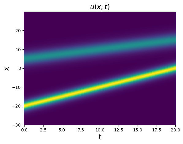
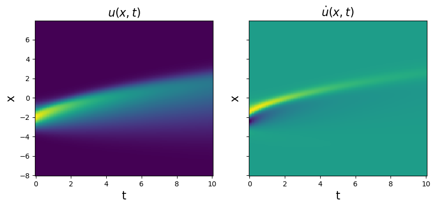
Test PDE functionality on the 1D kdV equation
The kdV equation is \(u_t = -6uu_x - u_{xxx}\), and the data we will be investigating is a two-soliton solution.
[4]:
# Load the data stored in a matlab .mat file
kdV = loadmat('data/kdv.mat')
t = np.ravel(kdV['t'])
x = np.ravel(kdV['x'])
u = np.real(kdV['usol'])
dt = t[1] - t[0]
dx = x[1] - x[0]
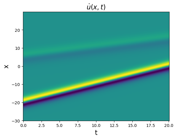
# Plot u and u_dot
plt.figure()
plt.pcolormesh(t, x, u)
plt.xlabel('t', fontsize=16)
plt.ylabel('x', fontsize=16)
plt.title(r'$u(x, t)$', fontsize=16)
plt.figure()
u_dot = ps.FiniteDifference(axis=1)._differentiate(u, t=dt)
plt.pcolormesh(t, x, u_dot)
plt.xlabel('t', fontsize=16)
plt.ylabel('x', fontsize=16)
plt.title(r'$\dot{u}(x, t)$', fontsize=16)
plt.show()
Test spatial derivative computations
[5]:
dx = x[1] - x[0]
ux = ps.FiniteDifference(d=1, axis=0,
                         drop_endpoints=False)._differentiate(u, dx)
uxx = ps.FiniteDifference(d=2, axis=0,
                          drop_endpoints=False)._differentiate(u, dx)
uxxx = ps.FiniteDifference(d=3, axis=0,
                           drop_endpoints=False)._differentiate(u, dx)
uxxxx = ps.FiniteDifference(d=4, axis=0,
                            drop_endpoints=False)._differentiate(u, dx)

# Plot derivative results
plt.figure(figsize=(18, 4))
plt.subplot(1, 4, 1)
plt.pcolormesh(t, x, ux)
plt.xlabel('t', fontsize=16)
plt.ylabel('x', fontsize=16)
plt.title(r'$u_x(x, t)$', fontsize=16)
plt.subplot(1, 4, 2)
plt.pcolormesh(t, x, uxx)
plt.xlabel('t', fontsize=16)
plt.ylabel('x', fontsize=16)
ax = plt.gca()
ax.set_yticklabels([])
plt.title(r'$u_{xx}(x, t)$', fontsize=16)
plt.subplot(1, 4, 3)
plt.pcolormesh(t, x, uxxx)
plt.xlabel('t', fontsize=16)
plt.ylabel('x', fontsize=16)
ax = plt.gca()
ax.set_yticklabels([])
plt.title(r'$u_{xxx}(x, t)$', fontsize=16)
plt.subplot(1, 4, 4)
plt.pcolormesh(t, x, uxxxx)
plt.xlabel('t', fontsize=16)
plt.ylabel('x', fontsize=16)
ax = plt.gca()
ax.set_yticklabels([])
plt.title(r'$u_{xxxx}(x, t)$', fontsize=16)
plt.show()
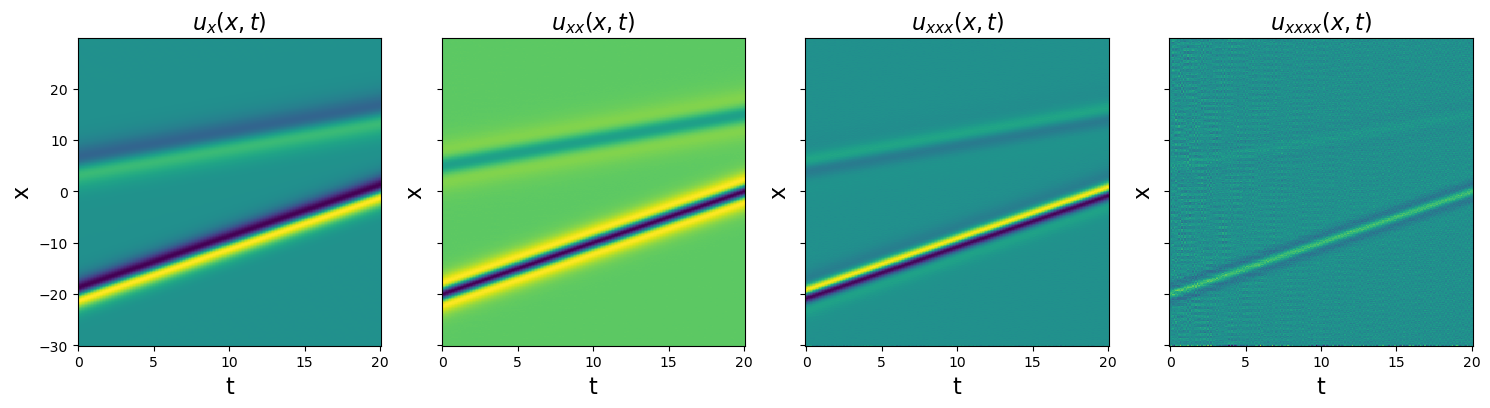
Note that the features get sharper and sharper in the higher-order derivatives, and any noise will be significantly amplified. Now we fit this data, and the algorithms struggle a bit.
[6]:
u = u.reshape(len(x), len(t), 1)

# Define PDE library that is quadratic in u, and
# third-order in spatial derivatives of u.
# library_functions = [lambda x: x, lambda x: x * x]
# library_function_names = [lambda x: x, lambda x: x + x]
pde_lib = ps.PDELibrary(function_library=ps.PolynomialLibrary(degree=2,include_bias=False),
                        derivative_order=3, spatial_grid=x,
                        include_bias=True, is_uniform=True)

# Fit the model with different optimizers.
# Using normalize_columns = True to improve performance.
print('STLSQ model: ')
optimizer = ps.STLSQ(threshold=5, alpha=1e-5, normalize_columns=True)
model = ps.SINDy(feature_library=pde_lib, optimizer=optimizer)
model.fit(u, t=dt)
model.print()

print('SR3 model, L0 norm: ')
optimizer = ps.SR3(threshold=7, max_iter=10000, tol=1e-15, nu=1e2,
                   thresholder='l0', normalize_columns=True)
model = ps.SINDy(feature_library=pde_lib, optimizer=optimizer)
model.fit(u, t=dt)
model.print()

print('SR3 model, L1 norm: ')
optimizer = ps.SR3(threshold=0.05, max_iter=10000, tol=1e-15,
                   thresholder='l1', normalize_columns=True)
model = ps.SINDy(feature_library=pde_lib, optimizer=optimizer)
model.fit(u, t=dt)
model.print()

print('SSR model: ')
optimizer = ps.SSR(normalize_columns=True, kappa=5e-3)
model = ps.SINDy(feature_library=pde_lib, optimizer=optimizer)
model.fit(u, t=dt)
model.print()

print('SSR (metric = model residual) model: ')
optimizer = ps.SSR(criteria='model_residual', normalize_columns=True, kappa=5e-3)
model = ps.SINDy(feature_library=pde_lib, optimizer=optimizer)
model.fit(u, t=dt)
model.print()

print('FROLs model: ')
optimizer = ps.FROLS(normalize_columns=True, kappa=1e-5)
model = ps.SINDy(feature_library=pde_lib, optimizer=optimizer)
model.fit(u, t=dt)
model.print()
STLSQ model:
(x0)' = -0.992 x0_111 + -5.967 x0x0_1
SR3 model, L0 norm:
(x0)' = -0.915 x0_111 + -5.682 x0x0_1
SR3 model, L1 norm:
(x0)' = -0.205 x0_1 + -0.728 x0_111 + -4.521 x0x0_1
SSR model:
(x0)' = -0.054 x0_1 + -0.918 x0_111 + -5.681 x0x0_1 + 0.290 x0^2x0_1
SSR (metric = model residual) model:
(x0)' = -0.054 x0_1 + -0.918 x0_111 + -5.681 x0x0_1 + 0.290 x0^2x0_1
FROLs model:
(x0)' = -0.069 x0_1 + -0.921 x0_111 + -5.540 x0x0_1
Note that improvements can be found by scanning over kappa until SSR and FROLs produce better models. But this highlights the liability of these greedy algorithms… they have weak and local convergence guarantees so for some problems they “make mistakes” as the algorithm iterations proceed.
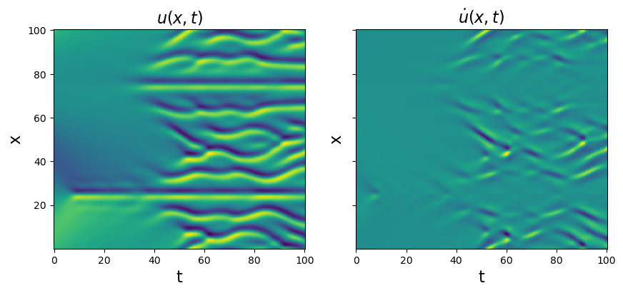
Test PDE functionality on the Kuramoto-Sivashinsky equation
The Kuramoto-Sivashinsky equation is \(u_t = -uu_x - u_{xx} - u_{xxxx}\). We will repeat all the same steps
[7]:
# Load data from .mat file
data = loadmat('data/kuramoto_sivishinky.mat')
t = np.ravel(data['tt'])
x = np.ravel(data['x'])
u = data['uu']
dt = t[1] - t[0]
dx = x[1] - x[0]

# Plot u and u_dot
plt.figure(figsize=(10, 4))
plt.subplot(1, 2, 1)
plt.pcolormesh(t, x, u)
plt.xlabel('t', fontsize=16)
plt.ylabel('x', fontsize=16)
plt.title(r'$u(x, t)$', fontsize=16)
u_dot = ps.FiniteDifference(axis=1)._differentiate(u, t=dt)

plt.subplot(1, 2, 2)
plt.pcolormesh(t, x, u_dot)
plt.xlabel('t', fontsize=16)
plt.ylabel('x', fontsize=16)
ax = plt.gca()
ax.set_yticklabels([])
plt.title(r'$\dot{u}(x, t)$', fontsize=16)
plt.show()

u = u.reshape(len(x), len(t), 1)
u_dot = u_dot.reshape(len(x), len(t), 1)
[8]:
train = range(0, int(len(t) * 0.6))
test = [i for i in np.arange(len(t)) if i not in train]
u_train = u[:, train, :]
u_test = u[:, test, :]
u_dot_train = u_dot[:, train, :]
u_dot_test = u_dot[:, test, 0]
t_train = t[train]
t_test = t[test]

# Define PDE library that is quadratic in u, and
# fourth-order in spatial derivatives of u.
# library_functions = [lambda x: x, lambda x: x * x]
# library_function_names = [lambda x: x, lambda x: x + x]
pde_lib = ps.PDELibrary(
#     library_functions=library_functions,
#     function_names=library_function_names,
    function_library=ps.PolynomialLibrary(degree=2,include_bias=False),
    derivative_order=4,
    spatial_grid=x,
    include_bias=True,
    is_uniform=True,
    periodic=True
)

# Again, loop through all the optimizers
print('STLSQ model: ')
optimizer = ps.STLSQ(threshold=10, alpha=1e-5, normalize_columns=True)
model = ps.SINDy(feature_library=pde_lib, optimizer=optimizer)
model.fit(u_train, t=dt)
model.print()
u_dot_stlsq = model.predict(u_test)

print('SR3 model, L0 norm: ')
optimizer = ps.SR3(
    threshold=7,
    max_iter=10000,
    tol=1e-15,
    nu=1e2,
    thresholder="l0",
    normalize_columns=True,
)
model = ps.SINDy(feature_library=pde_lib, optimizer=optimizer)
model.fit(u_train, t=dt)
model.print()

print('SR3 model, L1 norm: ')
optimizer = ps.SR3(
    threshold=1, max_iter=10000, tol=1e-15, thresholder="l1", normalize_columns=True
)
model = ps.SINDy(feature_library=pde_lib, optimizer=optimizer)
model.fit(u_train, t=dt)
model.print()

print('SSR model: ')
optimizer = ps.SSR(normalize_columns=True, kappa=1e1)
model = ps.SINDy(feature_library=pde_lib, optimizer=optimizer)
model.fit(u_train, t=dt)
model.print()

print('SSR (metric = model residual) model: ')
optimizer = ps.SSR(criteria="model_residual", normalize_columns=True, kappa=1e1)
model = ps.SINDy(feature_library=pde_lib, optimizer=optimizer)
model.fit(u_train, t=dt)
model.print()

print('FROLs model: ')
optimizer = ps.FROLS(normalize_columns=True, kappa=1e-4)
model = ps.SINDy(feature_library=pde_lib, optimizer=optimizer)
model.fit(u_train, t=dt)
model.print()
STLSQ model:
(x0)' = -0.995 x0_11 + -0.997 x0_1111 + -0.993 x0x0_1
SR3 model, L0 norm:
(x0)' = -0.993 x0_11 + -0.996 x0_1111 + -0.995 x0x0_1
SR3 model, L1 norm:
(x0)' = -0.791 x0_11 + -0.812 x0_1111 + -0.824 x0x0_1
SSR model:
(x0)' = -0.993 x0_11 + -0.997 x0_1111 + -0.993 x0x0_1 + -0.001 x0^2x0_11
SSR (metric = model residual) model:
(x0)' = -0.993 x0_11 + -0.997 x0_1111 + -0.993 x0x0_1 + -0.001 x0^2x0_11
FROLs model:
(x0)' = -0.995 x0_11 + -0.997 x0_1111 + -0.993 x0x0_1
[9]:
# Make fancy plot comparing derivative
plt.figure(figsize=(16, 4))
plt.subplot(1, 3, 1)
plt.pcolormesh(t_test, x, u_dot_test,
               cmap='seismic', vmin=-1.5, vmax=1.5)
plt.colorbar()
plt.xlabel('t', fontsize=20)
plt.ylabel('x', fontsize=20)
ax = plt.gca()
ax.set_xticks([])
ax.set_yticks([])

plt.subplot(1, 3, 2)
u_dot_stlsq = np.reshape(u_dot_stlsq, (len(x), len(t_test)))
plt.pcolormesh(t_test, x, u_dot_stlsq,
               cmap='seismic', vmin=-1.5, vmax=1.5)
plt.colorbar()
plt.xlabel('t', fontsize=20)
plt.ylabel('x', fontsize=20)
ax = plt.gca()
ax.set_xticks([])
ax.set_yticks([])

plt.subplot(1, 3, 3)
plt.pcolormesh(t_test, x, u_dot_stlsq - u_dot_test,
               cmap='seismic', vmin=-0.05, vmax=0.05)
plt.colorbar()
plt.xlabel('t', fontsize=20)
plt.ylabel('x', fontsize=20)
ax = plt.gca()
ax.set_xticks([])
ax.set_yticks([])
plt.show()
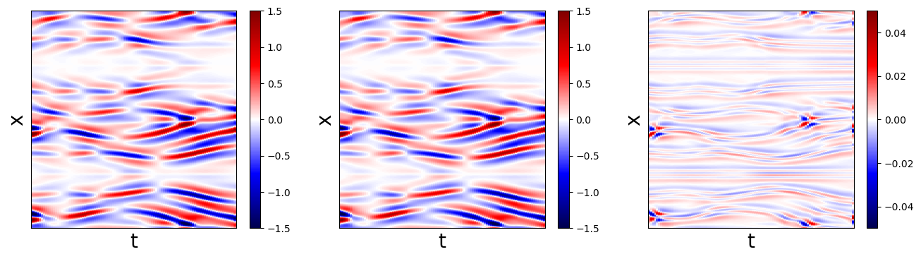
Interestingly, all the models perform quite well on the KS equation. Below, we test our methods on one more 1D PDE, the famous Burgers’ equation, before moving on to more advanced examples in 2D and 3D PDEs.
Test PDE functionality on Burgers’ equation
Burgers’ equation is \(u_t = -uu_x + 0.1 u_{xx}\). We will repeat all the same steps
[10]:
# Load data from .mat file
data = loadmat('data/burgers.mat')
t = np.ravel(data['t'])
x = np.ravel(data['x'])
u = np.real(data['usol'])
dt = t[1] - t[0]
dx = x[1] - x[0]

# Plot u and u_dot
plt.figure(figsize=(10, 4))
plt.subplot(1, 2, 1)
plt.pcolormesh(t, x, u)
plt.xlabel('t', fontsize=16)
plt.ylabel('x', fontsize=16)
plt.title(r'$u(x, t)$', fontsize=16)
u_dot = ps.FiniteDifference(axis=1)._differentiate(u, t=dt)

plt.subplot(1, 2, 2)
plt.pcolormesh(t, x, u_dot)
plt.xlabel('t', fontsize=16)
plt.ylabel('x', fontsize=16)
ax = plt.gca()
ax.set_yticklabels([])
plt.title(r'$\dot{u}(x, t)$', fontsize=16)
plt.show()

u = u.reshape(len(x), len(t), 1)
u_dot = u_dot.reshape(len(x), len(t), 1)
[11]:
# library_functions = [lambda x: x, lambda x: x * x]
# library_function_names = [lambda x: x, lambda x: x + x]
pde_lib = ps.PDELibrary(
#     library_functions=library_functions,
#     function_names=library_function_names,
    function_library=ps.PolynomialLibrary(degree=2,include_bias=False),
    derivative_order=3,
    spatial_grid=x,
    is_uniform=True,
)

print('STLSQ model: ')
optimizer = ps.STLSQ(threshold=2, alpha=1e-5, normalize_columns=True)
model = ps.SINDy(feature_library=pde_lib, optimizer=optimizer)
model.fit(u, t=dt)
model.print()

print('SR3 model, L0 norm: ')
optimizer = ps.SR3(
    threshold=2,
    max_iter=10000,
    tol=1e-15,
    nu=1e2,
    thresholder="l0",
    normalize_columns=True,
)
model = ps.SINDy(feature_library=pde_lib, optimizer=optimizer)
model.fit(u, t=dt)
model.print()

print('SR3 model, L1 norm: ')
optimizer = ps.SR3(
    threshold=0.5, max_iter=10000, tol=1e-15,
    thresholder="l1", normalize_columns=True
)
model = ps.SINDy(feature_library=pde_lib, optimizer=optimizer)
model.fit(u, t=dt)
model.print()

print('SSR model: ')
optimizer = ps.SSR(normalize_columns=True, kappa=1)
model = ps.SINDy(feature_library=pde_lib, optimizer=optimizer)
model.fit(u, t=dt)
model.print()

print('SSR (metric = model residual) model: ')
optimizer = ps.SSR(criteria="model_residual",
                   normalize_columns=True,
                   kappa=1)
model = ps.SINDy(feature_library=pde_lib, optimizer=optimizer)
model.fit(u, t=dt)
model.print()

print('FROLs model: ')
optimizer = ps.FROLS(normalize_columns=True, kappa=1e-3)
model = ps.SINDy(feature_library=pde_lib, optimizer=optimizer)
model.fit(u, t=dt)
model.print()
STLSQ model:
(x0)' = 0.100 x0_11 + -1.001 x0x0_1
SR3 model, L0 norm:
(x0)' = 0.100 x0_11 + -1.000 x0x0_1
SR3 model, L1 norm:
(x0)' = -0.032 x0_1 + 0.058 x0_11 + -0.700 x0x0_1
SSR model:
(x0)' = 0.100 x0_11 + -1.001 x0x0_1
SSR (metric = model residual) model:
(x0)' = 0.100 x0_11 + -1.001 x0x0_1
FROLs model:
(x0)' = 0.100 x0_11 + -1.001 x0x0_1
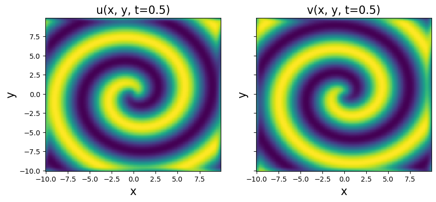
Test PDE functionality on 2D Reaction-Diffusion system
This 2D system is significantly more complicated. The reaction-diffusion system exhibits spiral waves on a periodic domain,and the PDEs are:
The main change will be a significantly larger library… cubic terms in (u, v) and all their first and second order derivatives. We will also need to generate the data because saving a high-resolution form of the data makes a fairly large file.
[12]:
from numpy.fft import fft2, ifft2
integrator_keywords['method'] = 'RK45'  # switch to RK45 integrator


# Define the reaction-diffusion PDE in the Fourier (kx, ky) space
def reaction_diffusion(t, uvt, K22, d1, d2, beta, n, N):
    ut = np.reshape(uvt[:N], (n, n))
    vt = np.reshape(uvt[N : 2 * N], (n, n))
    u = np.real(ifft2(ut))
    v = np.real(ifft2(vt))
    u3 = u ** 3
    v3 = v ** 3
    u2v = (u ** 2) * v
    uv2 = u * (v ** 2)
    utrhs = np.reshape((fft2(u - u3 - uv2 + beta * u2v + beta * v3)), (N, 1))
    vtrhs = np.reshape((fft2(v - u2v - v3 - beta * u3 - beta * uv2)), (N, 1))
    uvt_reshaped = np.reshape(uvt, (len(uvt), 1))
    uvt_updated = np.squeeze(
        np.vstack(
            (-d1 * K22 * uvt_reshaped[:N] + utrhs,
             -d2 * K22 * uvt_reshaped[N:] + vtrhs)
        )
    )
    return uvt_updated


# Generate the data
t = np.linspace(0, 10, int(10 / 0.05))
d1 = 0.1
d2 = 0.1
beta = 1.0
L = 20  # Domain size in X and Y directions
n = 128  # Number of spatial points in each direction
N = n * n
x_uniform = np.linspace(-L / 2, L / 2, n + 1)
x = x_uniform[:n]
y = x_uniform[:n]
n2 = int(n / 2)
# Define Fourier wavevectors (kx, ky)
kx = (2 * np.pi / L) * np.hstack((np.linspace(0, n2 - 1, n2),
                                  np.linspace(-n2, -1, n2)))
ky = kx
# Get 2D meshes in (x, y) and (kx, ky)
X, Y = np.meshgrid(x, y)
KX, KY = np.meshgrid(kx, ky)
K2 = KX ** 2 + KY ** 2
K22 = np.reshape(K2, (N, 1))

m = 1  # number of spirals

# define our solution vectors
u = np.zeros((len(x), len(y), len(t)))
v = np.zeros((len(x), len(y), len(t)))

# Initial conditions
u[:, :, 0] = np.tanh(np.sqrt(X ** 2 + Y ** 2)) * np.cos(
    m * np.angle(X + 1j * Y) - (np.sqrt(X ** 2 + Y ** 2))
)
v[:, :, 0] = np.tanh(np.sqrt(X ** 2 + Y ** 2)) * np.sin(
    m * np.angle(X + 1j * Y) - (np.sqrt(X ** 2 + Y ** 2))
)

# uvt is the solution vector in Fourier space, so below
# we are initializing the 2D FFT of the initial condition, uvt0
uvt0 = np.squeeze(
    np.hstack(
        (np.reshape(fft2(u[:, :, 0]), (1, N)),
         np.reshape(fft2(v[:, :, 0]), (1, N)))
    )
)

# Solve the PDE in the Fourier space, where it reduces to system of ODEs
uvsol = solve_ivp(
    reaction_diffusion, (t[0], t[-1]), y0=uvt0, t_eval=t,
    args=(K22, d1, d2, beta, n, N), **integrator_keywords
)
uvsol = uvsol.y

# Reshape things and ifft back into (x, y, t) space from (kx, ky, t) space
for j in range(len(t)):
    ut = np.reshape(uvsol[:N, j], (n, n))
    vt = np.reshape(uvsol[N:, j], (n, n))
    u[:, :, j] = np.real(ifft2(ut))
    v[:, :, j] = np.real(ifft2(vt))

# Plot to check if spiral is nicely reproduced
plt.figure(figsize=(10, 4))
plt.subplot(1, 2, 1)
plt.pcolor(X, Y, u[:, :, 10])
plt.xlabel('x', fontsize=16)
plt.ylabel('y', fontsize=16)
plt.title('u(x, y, t=0.5)', fontsize=16)
plt.subplot(1, 2, 2)
plt.pcolor(X, Y, v[:, :, 10])
plt.xlabel('x', fontsize=16)
plt.ylabel('y', fontsize=16)
ax = plt.gca()
ax.set_yticklabels([])
plt.title('v(x, y, t=0.5)', fontsize=16)

dt = t[1] - t[0]
dx = x[1] - x[0]
dy = y[1] - y[0]

u_sol = u
v_sol = v
[13]:
# Compute u_t from generated solution
u = np.zeros((n, n, len(t), 2))
u[:, :, :, 0] = u_sol
u[:, :, :, 1] = v_sol
u_dot = ps.FiniteDifference(axis=2)._differentiate(u, dt)

# Choose 60 % of data for training because data is big...
# can only randomly subsample if you are passing u_dot to model.fit!!!
train = np.random.choice(len(t), int(len(t) * 0.6), replace=False)
test = [i for i in np.arange(len(t)) if i not in train]
u_train = u[:, :, train, :]
u_test = u[:, :, test, :]
u_dot_train = u_dot[:, :, train, :]
u_dot_test = u_dot[:, :, test, :]
t_train = t[train]
t_test = t[test]
spatial_grid = np.asarray([X, Y]).T
[14]:
# Odd polynomial terms in (u, v), up to second order derivatives in (u, v)
# library_functions = [
#     lambda x: x,
#     lambda x: x * x * x,
#     lambda x, y: x * y * y,
#     lambda x, y: x * x * y,
# ]
# library_function_names = [
#     lambda x: x,
#     lambda x: x + x + x,
#     lambda x, y: x + y + y,
#     lambda x, y: x + x + y,
# ]
pde_lib = ps.PDELibrary(
#     library_functions=library_functions,
#     function_names=library_function_names,
    function_library=ps.PolynomialLibrary(degree=3,include_bias=False),
    derivative_order=2,
    spatial_grid=spatial_grid,
    include_bias=True,
    is_uniform=True,
    periodic=True
)
print('STLSQ model: ')
optimizer = ps.STLSQ(threshold=50, alpha=1e-5,
                     normalize_columns=True, max_iter=200)
model = ps.SINDy(feature_library=pde_lib, optimizer=optimizer)
model.fit(u_train, x_dot=u_dot_train)
model.print()
u_dot_stlsq = model.predict(u_test)

print('SR3 model, L0 norm: ')
optimizer = ps.SR3(
    threshold=60,
    max_iter=1000,
    tol=1e-10,
    nu=1,
    thresholder="l0",
    normalize_columns=True,
)
model = ps.SINDy(feature_library=pde_lib, optimizer=optimizer)
model.fit(u_train, x_dot=u_dot_train)
model.print()
u_dot_sr3 = model.predict(u_test)

print('SR3 model, L1 norm: ')
optimizer = ps.SR3(
    threshold=40,
    max_iter=1000,
    tol=1e-10,
    nu=1e2,
    thresholder="l1",
    normalize_columns=True,
)
model = ps.SINDy(feature_library=pde_lib, optimizer=optimizer)
model.fit(u_train, x_dot=u_dot_train)
model.print()

print('Constrained SR3 model, L0 norm: ')
feature_names = np.asarray(model.get_feature_names())
n_features = len(feature_names)
n_targets = u_train.shape[-1]
constraint_rhs = np.zeros(2)
constraint_lhs = np.zeros((2, n_targets * n_features))

# (u_xx coefficient) - (u_yy coefficient) = 0
constraint_lhs[0, 11] = 1
constraint_lhs[0, 15] = -1
# (v_xx coefficient) - (v_yy coefficient) = 0
constraint_lhs[1, n_features + 11] = 1
constraint_lhs[1, n_features + 15] = -1
optimizer = ps.ConstrainedSR3(
    threshold=.05,
    max_iter=400,
    tol=1e-10,
    nu=1,
    thresholder="l0",
    normalize_columns=False,
    constraint_rhs=constraint_rhs,
    constraint_lhs=constraint_lhs,
)
model = ps.SINDy(feature_library=pde_lib, optimizer=optimizer)
model.fit(u_train, x_dot=u_dot_train)
model.print()
u_dot_constrained_sr3 = model.predict(u_test)
STLSQ model:
(x0)' = 1.020 x0 + -1.020 x0^3 + 0.999 x0^2 x1 + -1.020 x0 x1^2 + 1.000 x1^3 + 0.101 x0_22 + 0.101 x0_11
(x1)' = 1.020 x1 + -1.000 x0^3 + -1.020 x0^2 x1 + -0.999 x0 x1^2 + -1.020 x1^3 + 0.101 x1_22 + 0.101 x1_11
SR3 model, L0 norm:
(x0)' = 1.019 x0 + -1.019 x0^3 + 0.998 x0^2 x1 + -1.017 x0 x1^2 + 0.998 x1^3 + 0.100 x0_22 + 0.101 x0_11
(x1)' = 1.019 x1 + -0.998 x0^3 + -1.017 x0^2 x1 + -0.998 x0 x1^2 + -1.019 x1^3 + 0.101 x1_22 + 0.101 x1_11
SR3 model, L1 norm:
(x0)' = 0.498 x0 + -0.446 x0^3 + 0.830 x0^2 x1 + -0.364 x0 x1^2 + 0.909 x1^3 + 0.018 x0_22 + 0.038 x0_11
(x1)' = 0.498 x1 + -0.909 x0^3 + -0.365 x0^2 x1 + -0.830 x0 x1^2 + -0.446 x1^3 + 0.037 x1_22 + 0.018 x1_11
Constrained SR3 model, L0 norm:
(x0)' = 1.016 x0 + -0.089 x1 + -1.009 x0^3 + 1.094 x0^2 x1 + -1.005 x0 x1^2 + 1.093 x1^3 + 0.092 x0_22 + 0.102 x0_11 + -0.063 x1^3x1_2 + -0.066 x0^2 x1x0_1 + 0.053 x1^3x1_1
(x1)' = 0.089 x0 + 1.016 x1 + -1.092 x0^3 + -1.005 x0^2 x1 + -1.093 x0 x1^2 + -1.009 x1^3 + 0.102 x1_22 + 0.092 x1_11 + -0.052 x0^3x0_2 + -0.067 x0 x1^2x1_2 + -0.063 x0^3x0_1
Takeaway: most of the optimizers can do a decent job of identifying the true system.
We skipped the greedy algorithms so this doesn’t run for too long. The constrained algorithm does okay, and correctly holds the constraints, but performance is limited currently because normalize_columns = True is crucial for performance here, but is not (currently) compatible with constraints.
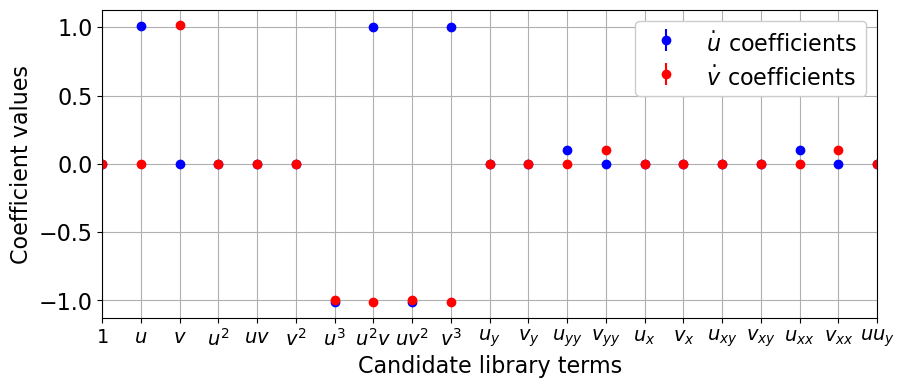
Below, we show that ensemble methods can generate excellent model identifications on 1/3 the data.
[20]:
# Show boosting functionality with 2D PDEs where 1/3 the data is used
optimizer = ps.STLSQ(threshold=40, alpha=1e-5, normalize_columns=True,unbias=False)
ensemble_optimizer = ps.EnsembleOptimizer(
    optimizer,
    bagging=True,
    n_models=10,
    n_subset=np.product(u_train.shape[:-1]) // 3,
)
model = ps.SINDy(feature_library=pde_lib, optimizer=ensemble_optimizer)
model.fit(u_train,
          x_dot=u_dot_train,
)
model.print()
(x0)' = 1.018 x0 + -1.018 x0^3 + 0.999 x0^2 x1 + -1.018 x0 x1^2 + 1.000 x1^3 + 0.101 x0_22 + 0.101 x0_11
(x1)' = 1.015 x1 + -1.000 x0^3 + -1.015 x0^2 x1 + -0.999 x0 x1^2 + -1.015 x1^3 + 0.101 x1_22 + 0.101 x1_11
[21]:
# Plot boosting results with error bars
xticknames = model.get_feature_names()
num_ticks = len(xticknames)
mean_coefs = np.mean(model.optimizer.coef_list, axis=0)
std_coefs = np.std(model.optimizer.coef_list, axis=0)
colors = ['b', 'r', 'k']
feature_names = ['u', 'v']
plt.figure(figsize=(10, 4))
for i in range(mean_coefs.shape[0]):
    plt.errorbar(range(mean_coefs.shape[1]),
                 mean_coefs[i, :], yerr=std_coefs[i, :],
                 fmt='o', color=colors[i],
                 label='$\dot ' + feature_names[i] + '_{}$' + ' coefficients')
ax = plt.gca()
ax.set_xticks(range(num_ticks))
for i in range(num_ticks):
    xticknames[i] = '$' + xticknames[i] + '$'
    xticknames[i] = xticknames[i].replace('x0', 'u')
    xticknames[i] = xticknames[i].replace('x1', 'v')
    xticknames[i] = xticknames[i].replace('_11', '_{xx}')
    xticknames[i] = xticknames[i].replace('_12', '_{xy}')
    xticknames[i] = xticknames[i].replace('_22', '_{yy}')
    xticknames[i] = xticknames[i].replace('_1', '_x')
    xticknames[i] = xticknames[i].replace('_2', '_y')
    xticknames[i] = xticknames[i].replace('uuu', 'u^3')
    xticknames[i] = xticknames[i].replace('uuv', 'u^2v')
    xticknames[i] = xticknames[i].replace('uuv', 'uv^2')
    xticknames[i] = xticknames[i].replace('vvv', 'v^3')

ax.set_xticklabels(xticknames)
plt.legend(fontsize=16, framealpha=1.0)
plt.xticks(fontsize=14)
plt.yticks(fontsize=16)
plt.grid(True)
plt.xlabel('Candidate library terms', fontsize=16)
plt.ylabel('Coefficient values', fontsize=16)
plt.xlim(0, 20)
plt.show()
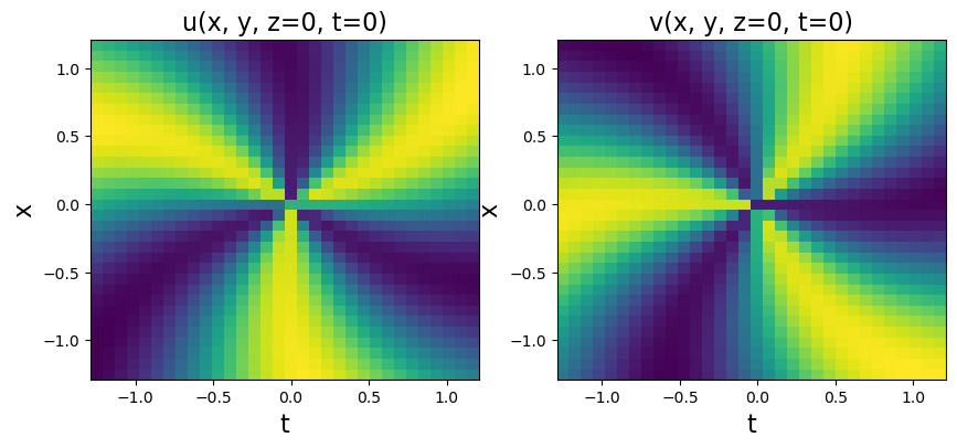
Test PDE functionality on 3D Reaction-Diffusion system
We will use a 3D reaction-diffusion equation called the Gray-Scott Equation. We are folllowing the example in Section 3.3.3 of Maddu, S., Cheeseman, B. L., Sbalzarini, I. F., & Müller, C. L. (2019). Stability selection enables robust learning of partial differential equations from limited noisy data. arXiv preprint arXiv:1907.07810., https://arxiv.org/pdf/1907.07810.pdf.
We will need to generate some very low-resolution data, because the memory requirements are very significant for a fully 3D problem. We will show below that with this very low-resolution data we can still approximately identify the PDE, but the weak form is required for further improvements (ensembling helps too but it doesn’t help the fact that the spatial resolution is so low).
[24]:
from numpy.fft import fftn, ifftn

# Define the reaction-diffusion PDE in the Fourier (kx, ky, kz) space
def reaction_diffusion(t, uvt, K22, d1, d2, n, N):
    ut = np.reshape(uvt[:N], (n, n, n))
    vt = np.reshape(uvt[N :2*N], (n, n, n))
    u = np.real(ifftn(ut, axes=[0, 1, 2]))
    v = np.real(ifftn(vt, axes=[0, 1, 2]))
    uv2 = u * (v ** 2)
    utrhs = np.reshape((fftn(0.014 * (1 - u) - uv2, axes=[0, 1, 2])), (N, 1))
    vtrhs = np.reshape((fftn(uv2 - 0.067 * v, axes=[0, 1, 2])), (N, 1))
    uvt_reshaped = np.reshape(uvt, (2 * N, 1))
    uvt_updated = np.squeeze(
        np.vstack(
            (-d1 * K22 * uvt_reshaped[:N] + utrhs,
             -d2 * K22 * uvt_reshaped[N:] + vtrhs)
        )
    )
    return uvt_updated


# Generate the data
dt = 0.1
t = np.linspace(0, 10, int(10 / dt))
d1 = 2e-2
d2 = 1e-2
L = 2.5  # Domain size in X, Y, Z directions

# use n = 32 for speed but then the high-order derivatives are terrible
n = 32  # Number of spatial points in each direction
N = n * n * n
x_uniform = np.linspace(-L / 2, L / 2, n + 1)
x = x_uniform[:n]
y = x_uniform[:n]
z = x_uniform[:n]
n2 = int(n / 2)
# Define Fourier wavevectors (kx, ky, kz)
kx = (2 * np.pi / L) * np.hstack((np.linspace(0, n2 - 1, n2),
                                  np.linspace(-n2, -1, n2)))
ky = kx
kz = kx
# Get 3D meshes in (x, y, z) and (kx, ky, kz)
X, Y, Z = np.meshgrid(x, y, z, indexing="ij")
KX, KY, KZ = np.meshgrid(kx, ky, kz, indexing="ij")
K2 = KX ** 2 + KY ** 2 + KZ ** 2
K22 = np.reshape(K2, (N, 1))

m = 3  # number of spirals

# define our solution vectors
u = np.zeros((len(x), len(y), len(z), len(t)))
v = np.zeros((len(x), len(y), len(z), len(t)))

# Initial conditions
u[:, :, :, 0] = np.tanh(np.sqrt(X ** 2 + Y ** 2 + Z ** 2)) * np.cos(
    m * np.angle(X + 1j * Y) - (np.sqrt(X ** 2 + Y ** 2 + Z ** 2))
)
v[:, :, :, 0] = np.tanh(np.sqrt(X ** 2 + Y ** 2 + Z ** 2)) * np.sin(
    m * np.angle(X + 1j * Y) - (np.sqrt(X ** 2 + Y ** 2 + Z ** 2))
)

# uvt is the solution vector in Fourier space, so below
# we are initializing the 2D FFT of the initial condition, uvt0
uvt0 = np.squeeze(
    np.hstack(
        (
            np.reshape(fftn(u[:, :, :, 0], axes=[0, 1, 2]), (1, N)),
            np.reshape(fftn(v[:, :, :, 0], axes=[0, 1, 2]), (1, N)),
        )
    )
)

# Solve the PDE in the Fourier space, where it reduces to system of ODEs
uvsol = solve_ivp(
    reaction_diffusion, (t[0], t[-1]), y0=uvt0, t_eval=t,
    args=(K22, d1, d2, n, N), **integrator_keywords
)
uvsol = uvsol.y

# Reshape things and ifft back into (x, y, z, t) space from (kx, ky, kz, t) space
for j in range(len(t)):
    ut = np.reshape(uvsol[:N, j], (n, n, n))
    vt = np.reshape(uvsol[N:, j], (n, n, n))
    u[:, :, :, j] = np.real(ifftn(ut, axes=[0, 1, 2]))
    v[:, :, :, j] = np.real(ifftn(vt, axes=[0, 1, 2]))

plt.figure(figsize=(10, 4))
plt.subplot(1, 2, 1)
plt.pcolor(X[:, :, 0], Y[:, :, 0], u[:, :, 0, 0])
plt.xlabel('t', fontsize=16)
plt.ylabel('x', fontsize=16)
plt.title('u(x, y, z=0, t=0)', fontsize=16)
plt.subplot(1, 2, 2)
plt.pcolor(X[:, :, 0], Y[:, :, 0], v[:, :, 0, 0])
plt.xlabel('t', fontsize=16)
plt.ylabel('x', fontsize=16)
plt.title('v(x, y, z=0, t=0)', fontsize=16)

dt = t[1] - t[0]
dx = x[1] - x[0]
dy = y[1] - y[0]
dz = z[1] - z[0]

u_sol = u
v_sol = v
[25]:
# Compute u_t from generated solution
u = np.zeros((n, n, n, len(t), 2))
u[:, :, :, :, 0] = u_sol
u[:, :, :, :, 1] = v_sol
u_dot = ps.FiniteDifference(axis=3)._differentiate(u, dt)

train = np.random.choice(len(t), int(len(t) * 0.6), replace=False)
test = [i for i in np.arange(len(t)) if i not in train]
u_train = u[:, :, :, train, :]
u_test = u[:, :, :, test, :]
u_dot_train = u_dot[:, :, :, train, :]
u_dot_test = u_dot[:, :, :, test, :]
t_train = t[train]
t_test = t[test]
spatial_grid = np.asarray([X, Y, Z])
spatial_grid = np.transpose(spatial_grid, [1, 2, 3, 0])
[33]:
library_functions = [
    lambda x: x,
    lambda x: x * x * x,
    lambda x, y: x * y * y,
    lambda x, y: x * x * y,
]
library_function_names = [
    lambda x: x,
    lambda x: x + x + x,
    lambda x, y: x + y + y,
    lambda x, y: x + x + y,
]
pde_lib = ps.PDELibrary(
    function_library=ps.CustomLibrary(library_functions=library_functions,function_names=library_function_names),
    derivative_order=2,
    spatial_grid=spatial_grid,
    include_bias=True,
    is_uniform=True,
    include_interaction=False,
    periodic=True
)

# optimizer = ps.SR3(threshold=5, normalize_columns=True,
#                    max_iter=5000, tol=1e-10)
optimizer = ps.STLSQ(alpha=1e-8, threshold=10, normalize_columns=True, unbias=False)
model = ps.SINDy(feature_library=pde_lib, optimizer=optimizer)
model.fit(u_train, x_dot=u_dot_train)
model.print()
(x0)' = 0.015 1 + -0.244 x0x0x0 + -1.342 x0x1x1 + 0.015 x0_22 + 0.019 x0_11
(x1)' = -0.038 x1 + -0.097 x1x1x1 + 1.130 x0x1x1 + -0.318 x0x0x1 + 0.012 x1_22 + 0.009 x1_11
[27]:
# Plot successful fits!
u_dot = model.predict(u_test)
u_dot = np.reshape(u_dot, (n, n, n, len(t_test), 2))

plt.figure(figsize=(10, 4))
plt.subplot(2, 2, 1)
plt.pcolor(X[:, :, 0], Y[:, :, 0], u_dot_test[:, :, 0, 1, 0])
plt.subplot(2, 2, 2)
plt.pcolor(X[:, :, 0], Y[:, :, 0], u_dot_test[:, :, 0, 1, 1])
plt.subplot(2, 2, 3)
plt.pcolor(X[:, :, 0], Y[:, :, 0], u_dot[:, :, 0, 1, 0])
plt.subplot(2, 2, 4)
plt.pcolor(X[:, :, 0], Y[:, :, 0], u_dot[:, :, 0, 1, 1])
plt.show()
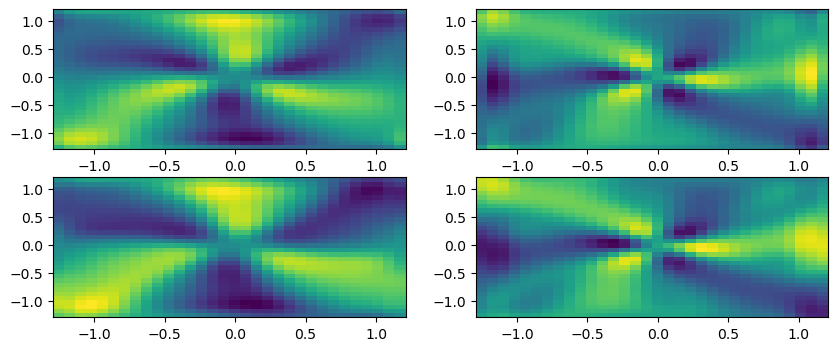
Despite the very low resolution, can do quite a decent job with the system identification!
We used only 50 timepoints and a 32 x 32 x 32 spatial mesh, and essentially capture the correct model for a 3D PDE!
[ ]: