In this notebook we address state space models for a plasma physics experiment
The HITSI-U experiment relies on a set of four injectors, each with three circuit variables. The model for the circuit is the following state space model:
The optimization problem solved for provably stable linear models is described further in example7_reboot.ipynb in this same folder.
![]()
[1]:
# import libraries
import numpy as np
import pysindy as ps
from matplotlib import pyplot as plt
from scipy.signal import StateSpace, lsim, dlsim
from scipy.io import loadmat
from sklearn.metrics import mean_squared_error
[2]:
# Define the state space model parameters
Amplitude = 600
Amplitude1 = 600
Frequency = 19000  # injector frequency
RunTime = .004
SampleTime = 1e-7
L1 = 8.0141e-7 # H
L2 = 2.0462e-6 # H
M = .161 * L2  # Coupling coefficient
Mw = .1346 * L2  # Coupling coefficient
Cap = 96e-6  # F
R1 = .0025  # Ohm
R2 = .005  # Ohm
R3 = .005  # Ohm
dT = 1e-7
PhaseAngle1 = 90
PhaseAngle2 = 180
PhaseAngle3 = 270

# Scale factor in front of the entries to the A matrix
# that are affected by mutual inductance
scalar1 = 1 / ((L2 - Mw) * ( (L2 ** 2) - (4 * M ** 2)  +  2 *L2 * Mw +  (Mw ** 2) ))
x3a =  (-L2 ** 2) * R2 + (2 * M ** 2) * R2 -L2 * Mw * R2
x3b = (-L2 ** 2) + (2 * M ** 2)-L2 * Mw
x3c = (L2 ** 2) * R2 - (2 * M ** 2) * R2 + L2 * Mw * R2 + (L2 ** 2) * R3 - (2 * M ** 2) * R3 + L2 * Mw * R3
x3d = L2 * M * R2 - M * Mw * R2
x3e = L2 * M- M * Mw
x3f = -L2 * M * R2 + M * Mw * R2 -L2 * M * R3 + M * Mw * R3
x3g = L2 * M * R2 - M * Mw * R2
x3h = L2 * M- M * Mw
x3i = -L2 * M * R2 + M * Mw * R2 -L2 * M * R3 + M * Mw * R3
x3j = - 2 * (M ** 2) * R2 + L2 * Mw * R2 + (Mw ** 2) * R2
x3k = - 2 * (M ** 2) + L2 * Mw + Mw ** 2
x3l = 2 * (M ** 2) * R2 -L2 * Mw * R2 - (Mw ** 2) * R2 + 2 * R3 * (M ** 2)-L2 * Mw * R3 - R3 * Mw ** 2

# Entries for x6 in A matrix
x6a = -L2 * M * R2 + M * Mw * R2
x6b = -L2 * M + M * Mw
x6c = L2 * M * R2 - M * Mw * R2 + L2 * M * R3 - M * Mw * R3
x6d = R2 * (L2 ** 2)- 2 * R2 * (M ** 2) + L2 * Mw * R2
x6e = (L2 ** 2)- 2 * (M ** 2) + L2 * Mw
x6f = - R2 * (L2 ** 2) + 2 * R2 * (M ** 2)-L2 * Mw * R2 - R3 * (L2 ** 2) + 2 * R3 * (M ** 2)-L2 * Mw * R3
x6g = 2 * R2 * (M ** 2)-L2 * Mw * R2 - R2 * (Mw ** 2)
x6h = 2 * (M ** 2)-L2 * Mw- (Mw ** 2)
x6i = - 2 * R2 * (M ** 2) + L2 * Mw * R2 + R2 * (Mw ** 2)- 2 * R3 * (M ** 2) + L2 * Mw * R3 + R3 * (Mw ** 2)
x6j = -L2 * M * R2 + M * Mw * R2
x6k = -L2 * M + M * Mw
x6l = L2 * M * R2 - M * Mw * R2 + L2 * M * R3 - M * Mw * R3

# Entries for x9 in A matrix
x9a = -L2 * M * R2  +  M * Mw * R2
x9b = -L2 * M  +  M * Mw
x9c = L2 * M * R2 - M * Mw * R2 *  +  L2 * M * R3  - M * Mw * R3
x9d = 2 * (M ** 2) * R2 - L2 * Mw * R2 - (Mw ** 2) * R2
x9e = 2 * (M ** 2) - L2 * Mw - (Mw ** 2)
x9f = - 2 * (M ** 2) * R2 +  L2 * Mw * R2  +  (Mw ** 2) * R2 - 2 * (M ** 2) * R3  +  L2 * Mw * R3  +  (Mw ** 2) * R3
x9g =(L2 ** 2) * R2 - 2 * (M ** 2) * R2  +  L2 * Mw * R2
x9h = (L2 ** 2) - 2 * (M ** 2)  +  L2 * Mw
x9i = - (L2 ** 2) * R2  +  2 * (M ** 2) * R2 - L2 * Mw * R2 - (L2 ** 2) * R3  +  2 * (M ** 2) * R3 - L2 * Mw * R3
x9j = -L2 * M * R2  +  M * Mw * R2
x9k = -L2 * M  +  M * Mw
x9l = L2 * M * R2 - M * Mw * R2  +  L2 * M * R3 - M * Mw * R3

#Entries for x12 in A matrix
x12a = - 2 * (M ** 2) * R2 +  L2 * Mw * R2  + (Mw ** 2) * R2
x12b = - 2 * (M ** 2)  +  L2 * Mw  +  (Mw ** 2)
x12c = 2 * (M ** 2) * R2 - L2 * Mw * R2 - (Mw ** 2) * R2  +  2 * (M ** 2) * R3 - L2 * Mw * R3 - (Mw ** 2) * R3
x12d = L2 * M * R2 - M * Mw * R2
x12e = L2 * M - M * Mw
x12f = -L2 * M * R2  +  M * Mw * R2 - L2 * M * R3  +  M * Mw * R3
x12g = L2 * M * R2 - M * Mw * R2
x12h = L2 * M - M * Mw
x12i = -L2 * M * R2  +  M * Mw * R2 - L2 * M * R3  +  M * Mw * R3
x12j = (-L2 ** 2) * R2  +  2 * (M ** 2) * R2 - L2 * Mw * R2
x12k = (-L2 ** 2)  +  2 * (M ** 2) - L2 * Mw
x12l = (L2 ** 2) * R2 - 2 * (M ** 2) * R2  +  L2 * Mw * R2  +  (L2 ** 2) * R3 - 2 * (M ** 2) * R3  +  L2 * Mw * R3
Finally, define the state space matrices
[3]:
A = np.array([[((-1 / L1) * (R1 + R2)), -1 / L1, R2 / L1, 0, 0, 0, 0, 0, 0, 0, 0, 0],
     [1 / Cap, 0, -1 / Cap, 0, 0, 0, 0, 0, 0, 0, 0, 0],
     [-scalar1 * x3a, -scalar1 * x3b,-scalar1 * x3c, -scalar1 * x3d,
      -scalar1 * x3e, -scalar1 * x3f, -scalar1 * x3g, -scalar1 * x3h,
      -scalar1 * x3i, -scalar1 * x3j, -scalar1 * x3k, -scalar1 * x3l],
     [0, 0, 0, ((-1 / L1)*(R1 + R2)), -1 / L1, R2*1 / L1, 0, 0, 0, 0, 0, 0],
     [0, 0, 0,  1 / Cap, 0, -1 / Cap, 0, 0, 0, 0, 0, 0],
     [scalar1 * x6a, scalar1 * x6b, scalar1 * x6c, scalar1 * x6d,
      scalar1 * x6e, scalar1 * x6f, scalar1 * x6g, scalar1 * x6h,
      scalar1 * x6i, scalar1 * x6j, scalar1 * x6k, scalar1 * x6l],
     [0, 0, 0, 0, 0, 0, ((-1 / L1) * (R1 + R2)), -1 / L1, R2 / L1, 0, 0, 0],
     [0, 0, 0, 0, 0, 0, 1 / Cap, 0, -1 / Cap, 0, 0, 0],
     [scalar1 * x9a, scalar1 * x9b, scalar1 * x9c, scalar1 * x9d,
      scalar1 * x9e, scalar1 * x9f, scalar1 * x9g, scalar1 * x9h,
      scalar1 * x9i, scalar1 * x9j, scalar1 * x9k, scalar1 * x9l],
     [0, 0, 0, 0, 0, 0, 0, 0, 0, ((-1 / L1) * (R1 + R2)), -1 / L1, R2 / L1],
     [0, 0, 0, 0, 0, 0, 0, 0, 0, 1 / Cap, 0, -1 / Cap],
     [-scalar1 * x12a, -scalar1 * x12b, -scalar1 * x12c, -scalar1 * x12d,
      -scalar1 * x12e, -scalar1 * x12f, -scalar1 * x12g, -scalar1 * x12h,
      -scalar1 * x12i, -scalar1 * x12j, -scalar1 * x12k, -scalar1 * x12l]]
)

B = np.array(
    [[1 / L1, 0, 0, 0],
    [0, 0, 0, 0],
    [0, 0, 0, 0],
    [0, 1 / L1, 0, 0],
    [0, 0, 0, 0],
    [0, 0, 0, 0],
    [0, 0, 1 / L1, 0],
    [0, 0, 0, 0],
    [0, 0, 0, 0],
    [0, 0, 0, 1 / L1],
    [0, 0, 0, 0],
    [0, 0, 0, 0]]
)

C = np.array(
    [[0,0,1, 0, 0, 0, 0, 0, 0, 0, 0, 0],
     [0, 0, 0, 0, 0, 1, 0, 0, 0, 0, 0, 0],
     [0, 0, 0, 0, 0, 0, 0, 0, 1, 0, 0, 0],
     [0, 0, 0, 0, 0, 0, 0, 0, 0, 0, 0, 1]]
)

D = np.zeros((C.shape[0], C.shape[0]))

sysc = StateSpace(A, B, C, D)
print(A.shape, C.shape, B.shape, D.shape)
print(np.linalg.eigvals(A))
(12, 12) (4, 12) (12, 4) (4, 4)
[-5374.04778628+128310.86801552j -5374.04778628-128310.86801552j
 -6150.9991369 +138653.66264826j -6150.9991369 -138653.66264826j
 -6044.9626724 +137273.04651637j -6044.9626724 -137273.04651637j
 -6044.96265483+137273.04655165j -6044.96265483-137273.04655165j
 -2052.57854051     +0.j         -2915.80444687     +0.j
 -2915.80453607     +0.j         -2983.64806906     +0.j        ]
Notice the A matrix has all negative eigenvalues, as it must!
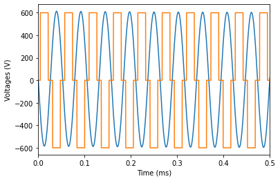
Load in the voltage control inputs
These are square waves at some pre-defined injector frequency.
[4]:
time = np.linspace(0, RunTime, int(RunTime / SampleTime) + 1, endpoint=True)
data = loadmat('data/voltages.mat')
voltage1 = data['voltage']
voltage2 = data['newVoltageShift1']
voltage3 = data['newVoltageShift2']
voltage4 = data['newVoltageShift3']
plt.plot(time * 1e3, voltage1)
plt.plot(time * 1e3, voltage3)
plt.xlim(0, 0.5)
plt.xlabel('Time (ms)')
plt.ylabel('Voltages (V)')
plt.show()
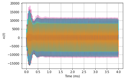
[5]:
tout, yout, xout = lsim(
    sysc,
    np.hstack([voltage1, voltage2, voltage3, voltage4]),
    time
)

# Add some noise proportional to the signal with the smallest amplitude of the 12
rmse = mean_squared_error(xout[:, 1], np.zeros(xout[:, 1].shape), squared=False)
xout = xout + np.random.normal(0, rmse / 100.0 * 0.1, xout.shape)  # add modest 0.1% noise

# Could consider rescaling units here
# xout = xout
# yout = yout
# tout = tout
# dt = tout[1] - tout[0]
for i in range(12):
    plt.plot(tout * 1000, xout[:, i])
plt.grid(True)
plt.xlabel('Time (ms)')
plt.ylabel(r'$x_i(t)$')
[5]:
Text(0, 0.5, '$x_i(t)$')
Discover the dx/dt = Ax + Bu part of the state space model
Try STLSQ instead – you will likely get an unstable model! Below we use a special optimizer to make sure the linear matrix is stable. \(\nu \ll 1\) promotes stability.
[6]:
# Define the control input
u = np.hstack([voltage1, voltage2, voltage3, voltage4])
sindy_library = ps.PolynomialLibrary(degree=1, include_bias=False)
optimizer_stable = ps.StableLinearSR3(
    threshold=0.0,
    thresholder='l1',
    nu=1e-5,
    max_iter=1000,
    tol=1e-5,
    verbose=True,
)

model = ps.SINDy(feature_library=sindy_library, optimizer=optimizer_stable)
model.fit(xout, t=tout, u=u)
/Users/alankaptanoglu/pysindy/pysindy/optimizers/stable_linear_sr3.py:200: UserWarning: This optimizer is set up to only be used with a purely linear library in the variables. No constant or nonlinear terms!
  "This optimizer is set up to only be used with a purely linear"
 Iteration ... |y - Xw|^2 ...  |w-u|^2/v ...       R(u) ... Total Error: |y - Xw|^2 + |w - u|^2 / v + R(u)
         0 ... 2.9958e+25 ... 1.7600e+18 ... 0.0000e+00 ... 2.9958e+25
       100 ... 2.9215e+25 ... 1.5349e+18 ... 0.0000e+00 ... 2.9215e+25
       200 ... 2.9215e+25 ... 1.5349e+18 ... 0.0000e+00 ... 2.9215e+25
       300 ... 2.9215e+25 ... 1.5349e+18 ... 0.0000e+00 ... 2.9215e+25
       400 ... 2.9215e+25 ... 1.5349e+18 ... 0.0000e+00 ... 2.9215e+25
       500 ... 2.9215e+25 ... 1.5349e+18 ... 0.0000e+00 ... 2.9215e+25
       600 ... 2.9215e+25 ... 1.5349e+18 ... 0.0000e+00 ... 2.9215e+25
       700 ... 2.9215e+25 ... 1.5349e+18 ... 0.0000e+00 ... 2.9215e+25
       800 ... 2.9215e+25 ... 1.5349e+18 ... 0.0000e+00 ... 2.9215e+25
       900 ... 2.9215e+25 ... 1.5349e+18 ... 0.0000e+00 ... 2.9215e+25
/Users/alankaptanoglu/pysindy/pysindy/optimizers/stable_linear_sr3.py:435: ConvergenceWarning: StableLinearSR3._reduce did not converge after 1000 iterations.
  ConvergenceWarning,
[6]:
SINDy(differentiation_method=FiniteDifference(),
      feature_library=PolynomialLibrary(degree=1, include_bias=False),
      feature_names=['x0', 'x1', 'x2', 'x3', 'x4', 'x5', 'x6', 'x7', 'x8', 'x9',
                     'x10', 'x11', 'u0', 'u1', 'u2', 'u3'],
      optimizer=StableLinearSR3(max_iter=1000, nu=1e-05, threshold=0.0,
                                verbose=True))
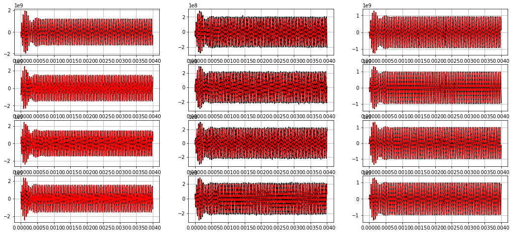
Without noise, can match A and B matrices quite well
[7]:
Xi = model.coefficients()
r = Xi.shape[0]
B_SINDy = Xi[:r, r:]
A_SINDy = Xi[:r, :r]

def normalized_error(matrix_true, matrix_pred):
    return np.linalg.norm(matrix_true - matrix_pred) / np.linalg.norm(matrix_true)

print(normalized_error(A, A_SINDy))
print(normalized_error(B, B_SINDy))
0.19068033430499962
0.20602516573898666
[8]:
ydot_true = model.differentiate(xout, t=tout)
ydot_pred = model.predict(xout, u=u)
plt.figure(figsize=(18, 8))
for i in range(12):
    plt.subplot(4, 3, i + 1)
    plt.grid(True)
    plt.plot(tout, ydot_true[:, i], 'k')
    plt.plot(tout, ydot_pred[:, i], 'r--')
Check if the A matrix is negative definite!
If not all the eigenvalues are negative, model is eventually unstable. If so, optimize with the StableLinearOptimizer until the eigenvalues are pushed to be all negative.
[9]:
Xi = model.coefficients()
print(np.sort(np.linalg.eigvals(Xi[:12, :12])))
[-7150.08962273     +0.j         -6363.42266396-136524.88261353j
 -6363.42266396+136524.88261353j -4538.98051827-131982.48166689j
 -4538.98051827+131982.48166689j -4051.1089204 -140910.1414539j
 -4051.1089204 +140910.1414539j  -3084.91951284     +0.j
 -2130.39210764-117766.90785961j -2130.39210764+117766.90785961j
 -1981.39239091  -2193.33083154j -1981.39239091  +2193.33083154j]
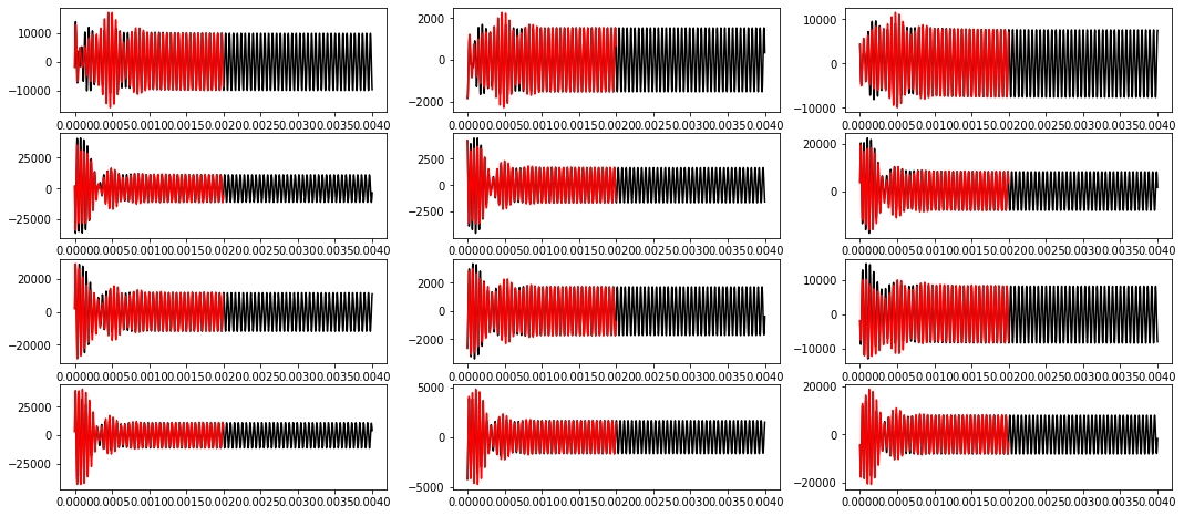
Now try resimulating the training data from some new initial condition
This is a 12D system and the time base is VERY well-sampled so integration might take a while!
[10]:
x0_new = (np.random.rand(12) - 0.5) * 10000
tout, yout, xout = lsim(
    sysc,
    u,
    time,
    X0=x0_new,
)
x_pred = model.simulate(
    x0_new,
    t=tout[:int(len(tout) // 2):10],
    u=u[:int(len(tout) // 2):10, :]
)
/Users/alankaptanoglu/pysindy/pysindy/pysindy.py:873: UserWarning: Last time point dropped in simulation because interpolation of control input was used. To avoid this, pass in a callable for u.
  "Last time point dropped in simulation because "
[11]:
plt.figure(figsize=(18, 8))
for i in range(12):
    plt.subplot(4, 3, i + 1)
    plt.plot(time, xout[:, i], 'k')
    plt.plot(tout[:int(len(tout) // 2) - 10:10], x_pred[:, i], 'r')